Links:
RHESSI Simulation Control Parameters
For a sample time, we'll use the flare of 4-jul-2002 06:20 UT
hsi_switch, /sim                                     ;true aspect -- simulate eventlist
o = hsi_eventlist(sim_ut_ref='4-jul-2002 06:22:36')  ;eventlist object
model = {gaussian_source_str}                        ;model structure
model.amplitude = 1.0                                ;Ignored, we're using separate source spectra
model.xysigma = [4.0, 4.0]                           ;Gaussian width
model.xypos = [-10.0, 0.0]                           ;10 arcsec from center
model = [model, model]                               ;Two sources
model[1].xypos = [10.0, 0.0]
spp = fltarr(6, 1, 2)                                ;6 components, 1 time profile, 2 sources
spp[*, 0, 0] = [0.049, 1.42, 1.0e-5, 6.0, 400.0, 6.0]   ;thermal, from OSPEX
spp[*, 0, 1] = [1.0e-5, 0.001, 1.35, 2.68, 13.72, 4.21] ;nonthermal, from OSPEX
o -> set, sim_spec_pars = spp                           ;set spectral pars
o -> set, sim_spec_model = 'f_vth_bpow'                 ;set spectral model
o -> set, /sim_use_spectrum                             ;use the spectrum input, the default is to simulate 50000 photons/subcollimator
o -> set, sim_background = 0                            ;no background (default)
o -> set, sim_xyoffset = [815.0, -325.0]                ;position between sources
o -> set, sim_model = model                             ;spatial model
o -> set, sim_energy_band = [3.0, 50.0]                 ;energy band, always a
                                                        ;good idea to go to 3 keV when doing
                                                        ;non-diagonal energy response
o -> set, sim_a2d_index_mask = [bytarr(9)+1]            ;The default

ev = o -> getdata(sim_time_range = [0.0, 24.0])         ;getdata
o -> Write, 'hsi_big_source_2.fits', time_range=[0, 0], energy_band=[0, 0]

; The [0,0]'s insure that all the data is written to the file
Here it turns out that the thermal and nonthermal sources have about the same number of photons.
Do 20 to 25 keV
hsi_switch, /flight
img_obj = hsi_image(ev_filename = 'hsi_big_source_2.fits')
image = img_obj -> getdata(xyoffset = [815.0, -325.0], $
                           energy_band = [20.0, 25.0], $
                           det_index_mask = [0, 0, 1, 1, 1, 1, 0, 1, 1], $
                           time_range = [0.0, 24.0], $
                           pixel_size = [1.0, 1.0])

img_obj -> set, image_alg = 'clean'
img_obj -> set_no_screen_output
image1 = img_obj -> getdata()

image2 = img_obj -> getdata(energy_band = [10.0, 15.0])
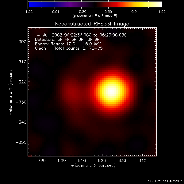
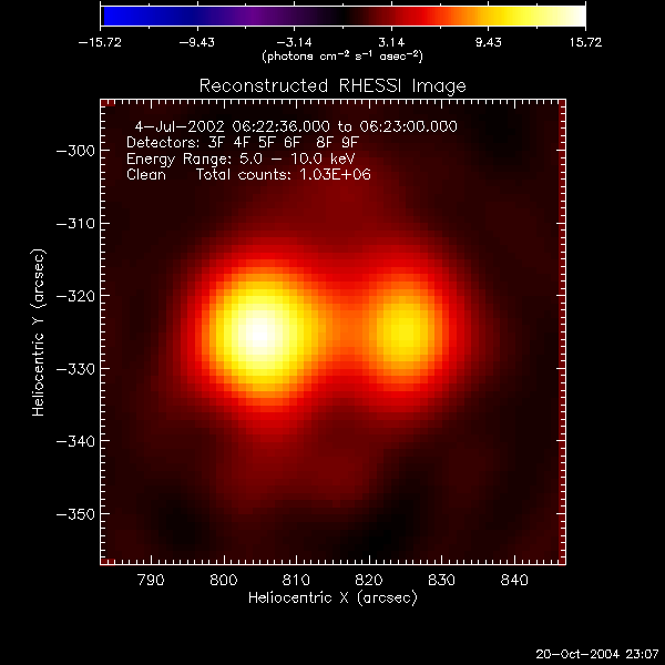
image3 = img_obj -> getdata(energy_band = [5.0, 10.0])
Put in thin attenuator, change time by 1 minute, keep the same spectrum. Now the nonthermal source has 10 times as many photons as the thermal.
hsi_switch, /sim
o = hsi_eventlist(sim_ut_ref='4-jul-2002 06:23:36')
model = {gaussian_source_str}
model.amplitude = 1.0
model.xysigma = [4.0, 4.0]
model.xypos = [-10.0, 0.0]
model = [model, model]
model[1].xypos = [10.0, 0.0]
spp = fltarr(6, 1, 2)
spp[*, 0, 0] = [0.049, 1.42, 1.0e-5, 6.0, 400.0, 6.0]
spp[*, 0, 1] = [1.0e-5, 0.001, 1.35, 2.68, 13.72, 4.21]
o -> set, sim_spec_pars = spp
o -> set, sim_spec_model = 'f_vth_bpow'
o -> set, /sim_use_spectrum
o -> set, sim_background = 0
o -> set, sim_xyoffset = [815.0, -325.0]
o -> set, sim_model = model
o -> set, sim_energy_band = [3.0, 50.0]
o -> set, sim_atten_state = 1                     ;May not have to set this?
ev = o -> getdata(sim_time_range = [0.0, 24.0])
o -> Write, 'hsi_big_source_3.fits', time_range=[0, 0], energy_band=[0, 0]
Same three image energy ranges


So in fact the nonthermal source dominates, but it isn't really only the +10 keV photons. Most of the nonthermal photons here are the extension of the spectrum below 10 keV:
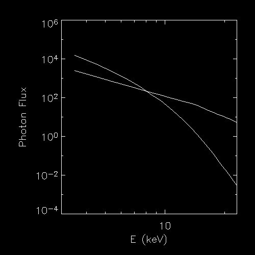
To demonstrate what we want, we need a sharp (if physically unrealistic) cutoff in the nonthermal flux.
energy = 3.0+findgen(98)
spp = fltarr(6, 1, 2)
spp[*, 0, 0] = [0.049, 1.42, 1.0e-5, 6.0, 400.0, 6.0]
spp[*, 0, 1] = [1.0e-5, 0.001, 1.35, 2.68, 13.72, 4.21]
pflux = fltarr(97, 1, 2) ;careful, vth gives flux at midpoints
pflux[*, 0, 0] = f_vth_bpow(energy, spp[*, 0, 0])
pflux[*, 0, 1] = f_vth_bpow(energy, spp[*, 0, 1])
pflux[0:6, 0, 1] = 1.0e-10
Instead of setting the spectral parameters, set the flux and energy
o -> set, sim_photon_flux = pflux
o -> set, sim_photon_energy = 0.5*(energy[1:*]+energy)

The 5 to 10 keV image still looks like the nonthermal source, but we *know* that these are photons that were generated at higher energy, but detected at 10 keV lower.

Comments to: jimm@ssl.berkeley.edu
21-Oct-2004, jmm