Weekly Report 20Aug2010
From RHESSI Wiki
Contents |
Visibility Forward Fit reduced chi2 and C statistics
In the following cases the visibility forward fit algorithm was used to make an image of a simulated point source at the center of the disk. The images were created allowing only a single iteration of the image fitting algorithm. This was done to check the effect on the reduced chi squared and C statistics of the image of varying either the full width half max of the source with all other parameters allowed to vary over only a single iteration or changing the flux of the image with all other parameters allowed to vary over only a single iteration. In both cases the initial guess for the source was a circular gaussian.
Visibility Forward Fit- reduced chi2 and C statistics when changing the FWHM of the circular source
In this case all parameters of the circular gaussian image were started at the values obtained by allowing the algorithm to iterate until it reached it's lowest reduced chi2 value. This was taken to be the best image the algorithm could create using a single circular gaussian source. All parameters except for the full width half max (FWHM) were started at these values. The FWHM was then systematically varied. The algorithm was allowed to do one iteration (see issues with visibility forward fit for an explanation of this)and the reduced chi2, the total C statistic, and the the C statistic for each detector were calculated.
The plot below shows the reduced chi2 as a function of the FWHM of the final image.
The reduced chi2 varies between a low of approximately 1.3 and a high of 1.6. The lowest point of the distribution is around a FWHM value of 2.5 arcsecs. The actual FWHM of the original image map is approximately 2 arcsecs so this seems to be a promising result. However at no point does the reduced chi2 reach the value of 0.87 achieved by allowing the algorithm to iterate.
The plot below shows the total C statistic of all detectors combined versus the final FWHM of the image.
The total C statistic is higher than the reduced chi2 in all cases. It is split into regions around 8 arcsecs. I do not understand the relationship between the C statistic and the reduced chi2 but the discontinuity seems very strange. If anyone has an explanation for this behavior please let me know.
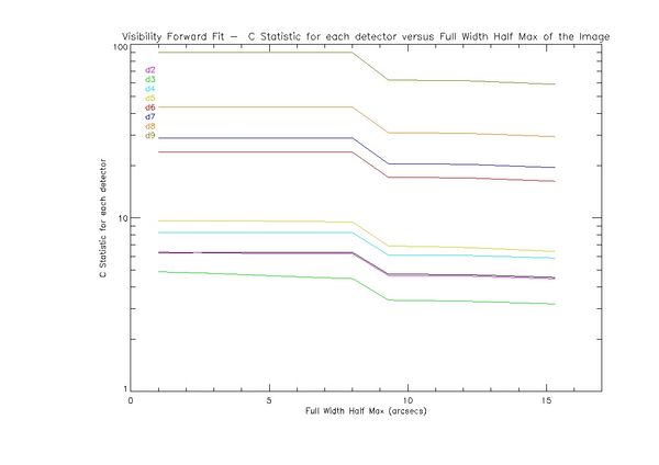
The plot below shows the C statistic for each individual detector as a function of the final FWHM of the image.
In the image above detector 1 is the black trace, it runs very close to detector 2 (purple). Once again the C statistic for all detectors are large compared to 1. The best of the group is detector 3. As the grids become coarser the C statistic becomes extremely bad with detector 9 being the worse, with C statistics close to 90. Once again each individual detector shows evidence of a discontinuity between 7 and 8 arcsecs. If the C statistic is an accurate measure of how well each detector fits the profile of the data then no detectors do a good job of fitting this source regardless of the FWHM of the image. The reduced chi2 looks to be misleading unless the C statistic is not a relevant measure of the probability of the image being accurate. Once again I'm not sure which is the better measure of the accuracy of the image.
Visibility Forward Fit - reduced chi2 and C statistics when changing the flux of the circular source
In the second case the best image parameters were once again used. This time the flux of the image was varied while all other parameters went through 1 iteration from their final values for the image with the lowest reduced chi2 after allowing the algorithm to iterate up to 2000 times.
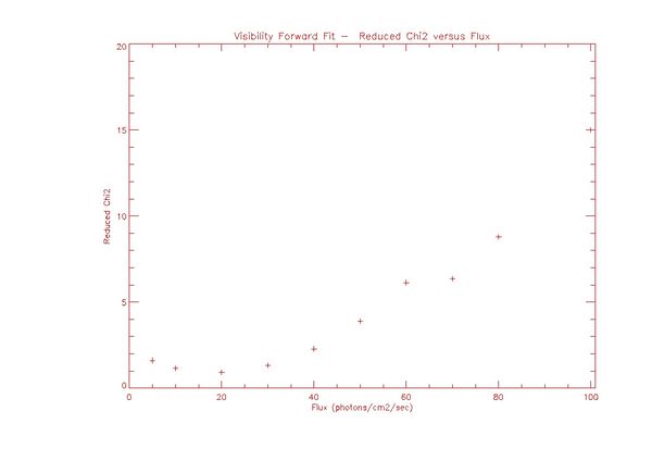
The plot below shows the reduced chi2 as a function of the final flux of the image
The reduced chi2 has it lowest value (approximately 1) around 20 photons/cm2/sec. As the value of the total flux is increased the reduced chi2 becomes a monotonically increasing function. Since the FWHM is the same for each image this displays that the visibility forward fit algorithm is sensitive to the photometry of the original source.
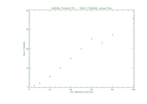
The plot below shows the total C statistic of the image as function of the total flux of the final image.
The total C statistic increases with the flux except for a slight dip at 70 ph/cm2/sec. This is odd since I expected a minimum at around the best value, but unlike the reduced chi2 this is not the case. Is this characteristic behavior of the C statistic, or is the explanation in the plot below, showing how quickly the C statistic in the detectors with coarser grids increases as a function of the total flux of the final image.
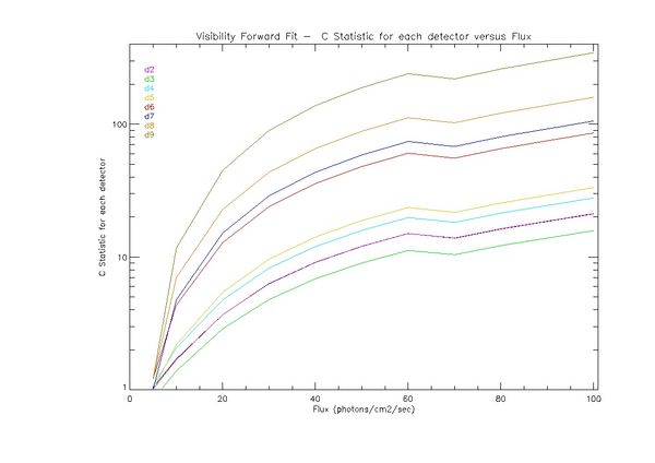
The plot below shows the C statistic of each detector as a function of the total flux in the final image.
Once again detector 1 is the black line that lays right along detector 2 (purple). The C statistic for each detector increases as a function of flux with no minimum at the value of around 20 ph/cm2/sec where the lowest reduced chi2 was found. The value of the C statistic in the detectors with coarser grids increases faster with an increase in flux than in the detectors with finer grids. This all leads back to the question of whether the reduced chi2 or the C statistic is a better measure of how good the image is and the relation between the two.
Issues with Visibility Forward Fit as Currently Implemented
Below are some issues encountered while using visibility forward fit.
- When iterations are set to 0 the algorithm still does 1 iteration, this meant that all parameters could not be fixed except for the one being studied because they would change slightly with the first iteration.
- When trying to use the previous fit as starting parameters for the next fit the program crashes, Kim Tolbert is looking at this problem.
- When changing from an elliptical gaussian to a circular gaussian the fit to the circular gaussian appears to use the elliptical parameters when fitting the visibilities but the the image appears circular. I'll confirm that this is consistent feature and try to track it down next week.
Assisted Weijung Liu with doing spectral fits using OSPEX
Assisted visiting graduate student Weijung Liu of Montana State University with doing spectral fits of a RHESSI flare. Explained using the drm_mod and pileup_mod fit components to improve the fits and get more accurate measurements of the physical parameters from the thermal and thick target fit components. I also showed her how to create single detector spectral files with native energy bins using an ssw routine.
Goals for next week
- Continue with the C statistic work on visibility forward fit. I'll need to talk to Brian about the above results and decide on the next course of action.
- Finish my IDL program for comparing algorithms to original simulated data maps by calculating the difference between the two, pixel by pixel. This is it's current state.
- Order a new hard drive for wilco as the sswdb is filling up the original drive.
- Try the image difference program to compare simulations and reconstructed images on the five maps I have available.


