Weekly Report 3Sep2010
From RHESSI Wiki
Contents |
Visibility Forward Fit - Elliptical Model
For the following tests an eventlist for a simulated point source at disk center was used. The visibility forward fit model used to create the image was an elliptical source. In both cases below the flux was help fixed. In the first case all parameters except for the flux were allowed to vary. In the second case all parameters except for the flux and the eccentricity of the ellipse were allowed to vary. The second case was carried out due to issues with the first case, as will be discussed below.
In all cases the measured visibility amplitude is the set shown below. The red curve is the best fit to these visibilities using an elliptical model with all parameters free. In the cases were the flux is fixed the fit to the visibilities is constrained and cannot achieve this optimal fit.
Visibility Forward Fit - Elliptical Model(Flux fixed all other parameters free)
In this case the flux was fixed and the other parameters of the elliptical model were allowed to vary. At the point were the reduced chi2 reached it's lowest value it was recorded along with the total C statistic and the C statistic for each detector from the image object.
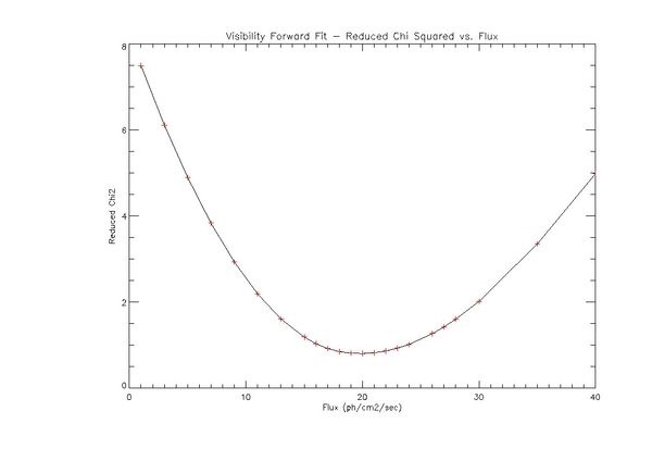
The plot below shows the value of the reduced chi2 as a function of the flux.
The reduced chi2 is a well behaved function of the flux. It has a single minimum at approximately 20ph/cm2/sec, around the same point as the the circular gaussian. Once again the reduced chi2 increases rapidly as the flux moves from the value that produces the minimum in the reduced chi2.
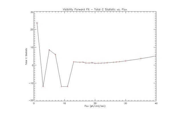
The plot below shows the total C statistic as a function of the flux.
The most noticeable feature of the plot are the points where the C statistic drops to approximately -12. Further exploration of these points showed that the eccentricity of the ellipse was very close to 1, however reviewing the C statistic with Richard Schwartz and Kim Tolbert showed that it should not become negative in this situation, but rather get large. I need to spend more time looking at these points, and the behavior of the C statistic in general. Ignoring those points, the curve of the C statistic looks similar to the curve for a circular gaussian model, although around the minimum it is flatter as the value of the flux increases. With the elliptical model it more difficult to identify the minimum as a function of flux. This is probably due to the extra free parameters in the elliptical gaussian. The FWHM and eccentricity can both be adjusted to help the fit, instead of just the FWHM. That said, I am puzzled as to why this would not show up just as prominently in the reduced chi2.
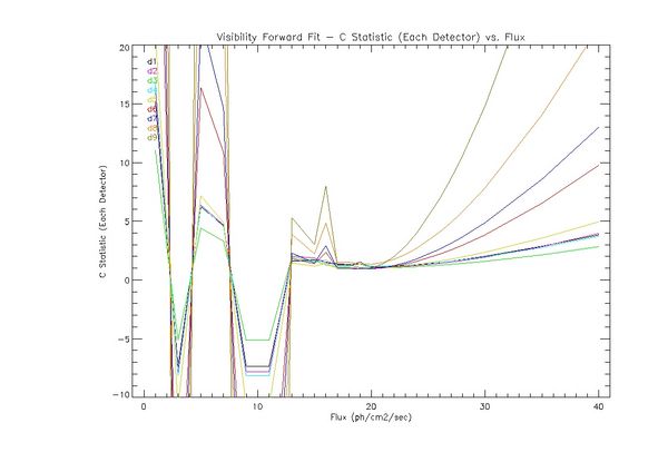
The plot below shows the C statistic for each detector as a function of flux.
Below 20 ph/cm2/sec the C statistic for each detector behaves erratically, dropping and rising quickly as the value of the flux is changed. At around 20 ph/cm2/sec the C statistics behave more smoothly and begin to rise. It seems that when there are too many free parameters visibility forward fit has a difficult time deciding on how to iterate the parameters to go towards the best fit.
Consequently the next test was trying the image reconstruction with fewer free parameters.
Visibility Forward Fit - Elliptical Model (Flux and Eccentricity fixed all other parameters free)
In the following test the flux and eccentricity of the elliptical gaussian were fixed. The flux was fixed at various values while the eccentricity was held fixed at .5. All the other parameters of the elliptical model were allowed to vary. When the final image was made at the lowest value of the reduced chi2, the reduced chi2, the total C statistic, and the C statistic for each detector were recorded.
The plot below shows the reduced chi2 as a function of the flux with the eccentricity of the model held fixed at .5
Once again the reduced chi2 behaves reasonably, with a single minimum at approximately 20 ph/cm2/sec and a sharp rise when the flux is lower or higher than the value at the minimum. The minimum is in the same place as the minimum with the eccentricity as a free parameter and has the same value of the reduced chi2.
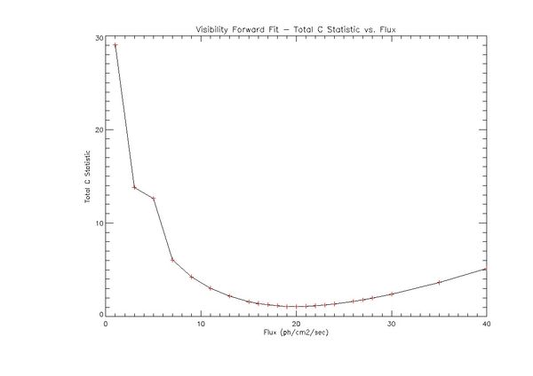
The plot below shows the total C statistic as a function of the flux with the eccentricity of the elliptical source held fixed at .5.
This curve looks much more well behaved than the the curve with the eccentricity as a free parameter. There is a shift between 3 and 5 ph/cm2/sec, a region that corresponds to where the image with eccentricity as a free parameter had a negative C statistic. This seems to be further evidence that visibility forward fit has trouble if there are too many free parameters. Once again the rise of the curve from the minimum is not as sharp when the flux is increased.
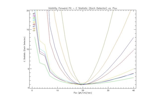
The curve below shows the C statistic for each detector as a function of the flux with a fixed eccentricity of .5.
The C statistic for each detector shows a minimum at around 20ph/cm2/sec, however the detectors with the finer grids and more visibilities show a kink between 3 and 5 ph/cm2/sec. I'll have to look more closely at what happens with these detectors there. Once again, as with the circular model the dominance of detectors with the finer grids and the algorithms attempt to fit these preferentially leads to a lower C statistic than would be expected.
Difference Plots - Model v. Reconstructed Image
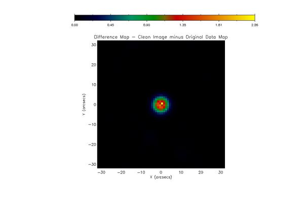
The image difference procedure was tested with a point source eventlist and the original data map. It was tested with several different methods of taking the difference between the images. The one shown below is a method with the original data map modified using congrid so it becomes mapped into pixels the same size as the image. A pixel by pixel subtraction was done. The difference was squared and then the square root of this value was taken to ensure all points were positive. In this case the difference looks very much like a point source. I think this is because the original data map and the reconstructed image are not in the same units so the calibration between the two is off. Can anyone help me with how to figure out this calibration?
New RHESSI Website
Continued importing content to the new RHESSI Website. Currently I am trying to figure out the best way to import and manage pages in typo3, the content management system we are now using. I am also working on a document on how to do this for other local users of the site to make it easier for them to add and edit content.
Goals for next week
- Continue with exploration of C statistic. Try to understand why the elliptical model can yield negative values. I'm going to create test data and run it through the routine we use to detrmine the C statistic to check on whether it is possible to get a negative C statistic.
- Work on importing more content to RHESSI site and on a typo3 guide for RHESSI site editors
- Check calibration problems with image difference program, calculate a weighted average of the map so we have a single number to compare each image we make with different algorithms and parameters.


