View fit results
From RHESSI Wiki
| Line 21: | Line 21: | ||
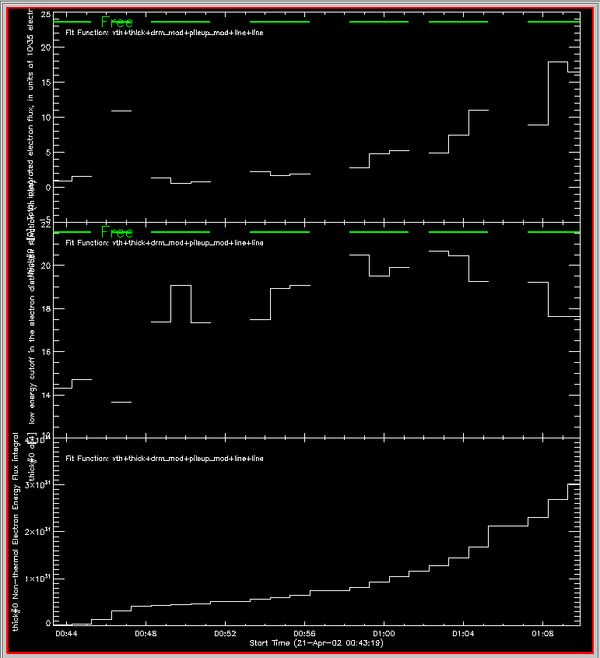
The green bar at the top of the the upper and middle panels show which time intervals were fit with the parameter free. This is useful in cases were the same parameters were not allowed to vary for all time intervals fit. The lower panel shows the integrated non-thermal electron energy flux. Note that the fill gaps option was used when doing the integration, hence the non-thermal electron energy has values even in time intervals when no fit was done. These values are estimates based doing a linear interpolation of the time intervals were a fit was done and the non-thermal electron energy flux could be calculated. | The green bar at the top of the the upper and middle panels show which time intervals were fit with the parameter free. This is useful in cases were the same parameters were not allowed to vary for all time intervals fit. The lower panel shows the integrated non-thermal electron energy flux. Note that the fill gaps option was used when doing the integration, hence the non-thermal electron energy has values even in time intervals when no fit was done. These values are estimates based doing a linear interpolation of the time intervals were a fit was done and the non-thermal electron energy flux could be calculated. | ||
| + | [[Category:Software]] | ||
Latest revision as of 00:31, 12 September 2009
View Fit Results
Introduction
This GUI allows the user to view the fit results for different parameters when multiple time intervals have been fit. It displays the parameters as a function of time or interval number with calculated error bars (showing statistical error) depending on the options selected by the user. If also has functionality that allows the display of the reduced χ2 as well as various properties of any given time interval, such as the model photon flux, the data photon flux, or the residuals.
Using View Fit Results
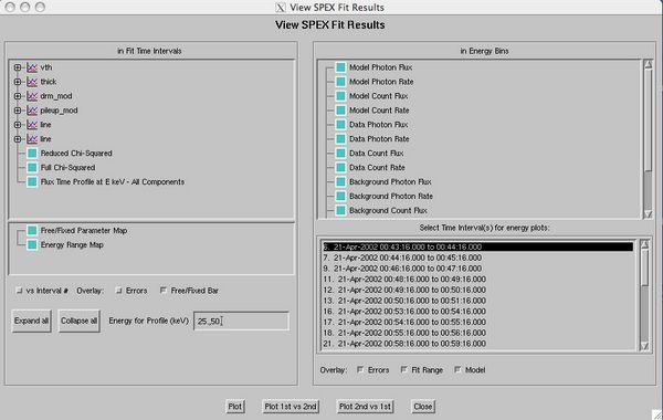
To view your fit results after fitting multiple intervals select the Plot Fit Results... option from the File drop down menu in the main OSPEX GUI window. The Fit Results GUI should appear:
The Fit Results GUI has several panels. The in Fit Time Intervals panel on the upper left displays the tree of components used for the fit along with the reduced and full χ2. It also contains an option for displaying the Flux Time profile at any given energy. Each component of the fit can be expanded to show it's individual components, for example expanding vth by clicking on the plus sign next to component name will show a list of the parameters of the function. In this case the a[0], the Emission Measure, a[1], the Temperature, and a[2], the relative abundance. There is also a button for the Flux time profile at a given energy for this component (vth in this case). Any component that has been allowed to vary during any saved fit will have a light blue box next to it, any that have not been allowed to vary for any fits will be grey. Selecting any of the components will show a plot of the component as a function of time in the main OSPEX GUI. The user can also select to view the results as function of interval number by selecting that option from the buttons on the lower left.
An important feature of the thick target or thick target 2 component is an additional button when the component is expanded that allows the plotting of the non-thermal electron energy flux. This is important because it means that there is now a way to go directly from doing RHESSI fits with a thick target model to calculating the energy in the non-thermal electrons very simply. Once fits have been done over the entire flare the user can plot the non-thermal electron flux from the thick target component. Using the XY Plot Options... button under the Plot_Control drop down menu, will bring the the UT Plot Options GUI up. Selecting the integral option from the Y axis options list will integrate the flux with respect to time. Subtracting the value of the integrated curve at the latest time from the earliest time will yield the total non-thermal energy over the time the flare was analyzed. Note that there is also a fill gaps button below the Y axis options. Selecting this will fill in the gaps for times when no fit was done so no non-thermal electron flux could be calculated. A linear interpolation is performed to calculate the value of the non-thermal electron flux at these points. This is more accurate than leaving gaps in data because it a more realistic model to say that some flux is present than zero when doing the integration.
The Flux Time Profile at E keV will give a flux profile at any selected energy as a function of time for the model. Select the energy on the lower left of the GUI by typing it into the energy for Profile (keV) box. Note that multiple energies can be selected by entering them in a comma separated list. Selecting the flux time profile at the bottom of the tree below the full χ2 option will show the flux at the energies selected for all components of the model combined. For instance if looking at a model of vth + thick target, this option will show the flux profile at a selected energy for the components added together as a function of time. To view the flux profile at a specific energy for a single component select the flux time profile at E option from the bottom of the list of component parameters after expanding the tree in the upper left panel.
The right side of the View Fit Results GUI lists options for viewing properties of fit dones in individual time intervals as a function of energy in keV. The lower right panel is used to select the time interval to view. Multiple time intervals can be selected. The upper right panel contains the possible choices of properties to view for each time interval as a function of Energy. If more than one interval is selected all traces are overlayed on the same plot. For instance selecting Model Photon Flux will show a plot of the photon flux derived from the model parameters as a function of energy for all time intervals selected. Only time intervals that have associated saved fits will be present in the Select Time Interval(s) list
The plot below shows two parameters from a fit using thick target along with the integrated non-thermal electron flux.

The green bar at the top of the the upper and middle panels show which time intervals were fit with the parameter free. This is useful in cases were the same parameters were not allowed to vary for all time intervals fit. The lower panel shows the integrated non-thermal electron energy flux. Note that the fill gaps option was used when doing the integration, hence the non-thermal electron energy has values even in time intervals when no fit was done. These values are estimates based doing a linear interpolation of the time intervals were a fit was done and the non-thermal electron energy flux could be calculated.
