Weekly Report 13Aug2010
From RHESSI Wiki
| (8 intermediate revisions not shown) | |||
| Line 9: | Line 9: | ||
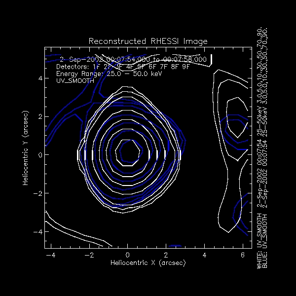
[[Image:Clean blue center white limb.jpg|center|thumb|600px|Contours of two clean images. The blue contours are the clean image of a point source with albedo at disk center. The white contours are a clean image of point source with albedo near the limb. It has has been translated to disk center so the 90% contour matches the 90% contour of the image at disk center. Detectors 1 thru 4 were used to create both images.]] | [[Image:Clean blue center white limb.jpg|center|thumb|600px|Contours of two clean images. The blue contours are the clean image of a point source with albedo at disk center. The white contours are a clean image of point source with albedo near the limb. It has has been translated to disk center so the 90% contour matches the 90% contour of the image at disk center. Detectors 1 thru 4 were used to create both images.]] | ||
| + | |||
| + | Using detectors 1 - 4, then translating the image of the source near the limb to disk center, we can observe that the 90 % contour to the 30% contour match for both images. The contours for the image at the center extend toward the limb as they go down in level. The image created for the source on the limb does not show foreshortening in along the North - South Heliocentric Y axis. Using the Clean imaging algorithm it is not possible to see the small structure (2 arcsecs and below) differences in the compact source near the limb versus at disk center. The lower level contours do show a distortion toward the disk center for the source near the limb, however I can't determine if this is due to the low number of counts away from the compact source or if it is a demonstration of the displacement of the extended source toward the center of the disk. | ||
| + | |||
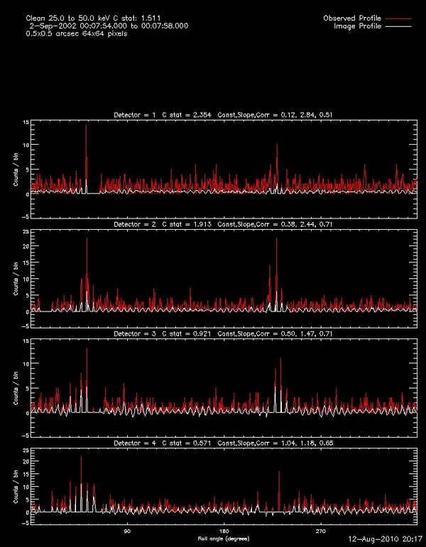
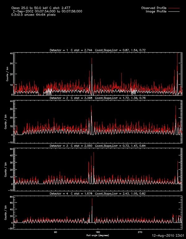
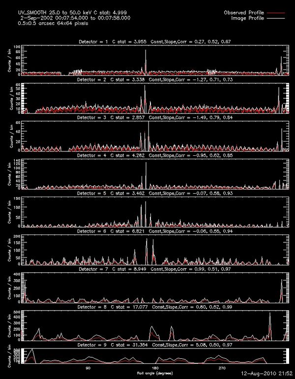
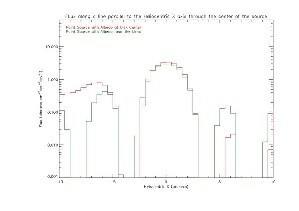
| + | The two plots below show the profiles of the the two images. The red curves are the observed data, the white curves are the fits to that data. The first plot shows the profiles of the image at disk center. The second plot shows the profiles of the image near the limb. | ||
[[Image:Clean profiles d1 d4 center.jpg|center|thumb|600px|The profiles of the data in each detector used to create the image at disk center along with the fits to those profiles. The data is shown in roll bins.]] | [[Image:Clean profiles d1 d4 center.jpg|center|thumb|600px|The profiles of the data in each detector used to create the image at disk center along with the fits to those profiles. The data is shown in roll bins.]] | ||
| Line 14: | Line 18: | ||
[[Image:Clean profiles d1 d4 limb.jpg|center|thumb|600px|The profiles of each detector used to create the image near the limb along with the fits to those profiles. The data is shown in roll bins.]] | [[Image:Clean profiles d1 d4 limb.jpg|center|thumb|600px|The profiles of each detector used to create the image near the limb along with the fits to those profiles. The data is shown in roll bins.]] | ||
| + | The profiles for both images show a bad fit for detectors 1 and 2. The C statistic in each case is over 2.0. This may be a result of the inability of the finer grids to image a source which is extended due to the albedo contribution, but I'm not sure. | ||
| + | For detectors 3 and 4 the fits for the image at disk center are good, they each have a C statistic below 1. For the image near the limb the C statistics are above 1. This implies that when the extended albedo source is displaced from the point source detectors 3 and 4 still have trouble imaging both sources while for a source at the center they can create a good image. The caveat to this conclusion is the pointsource and albedo at the center has 1/3 as many total counts as the one on the limb, so this may be a function of bad statistics. | ||
| + | |||
| + | |||
| + | The plot below shows the profiles along a line parallel to the Heliocentric X axis through the source for both images. The source near the limb has been translated so the peak matches the peak at disk center. It has also been normalized so the peak of the profile on the limb matches the flux of the peak at disk center. This was done to make direct comparison of the two profiles easier visually. The red curve is the profile of the image of the source at disk center. The green curve is the profile of the source near the limb. | ||
[[Image:Clean d1 d4 limb center profile.jpg|center|thumb|600px|The Flux profiles of each image along a line parallel to the Heliocentric X axis passing through the peak of the source. The red curve is the profile of the image at disk center. The green curve is the profile of the image near the limb. Note the green curve has been divided by a constant so the peak value is near the peak value of the red curve. It has also been translated to disk center. This was done to make it easier to compare the features of the two curves.]] | [[Image:Clean d1 d4 limb center profile.jpg|center|thumb|600px|The Flux profiles of each image along a line parallel to the Heliocentric X axis passing through the peak of the source. The red curve is the profile of the image at disk center. The green curve is the profile of the image near the limb. Note the green curve has been divided by a constant so the peak value is near the peak value of the red curve. It has also been translated to disk center. This was done to make it easier to compare the features of the two curves.]] | ||
| + | As expected from the contours the profiles match well at the peak off the profile. The distortion in the contours of the image near the limb toward the center are not significant enough to show up in this plot because the levels of those contours are low, however the distortion in the contours of the image at the center toward the limb do appear as an approximately 20% difference toward the limb. This may be a result of only using detectors 1 - 4. This is something I will explore further. | ||
| + | |||
| + | |||
====Pixon==== | ====Pixon==== | ||
| + | The following plot shows the contours of an image for a point source at the center of the disk created using Pixon with detectors 1 -4 compared with a point source near the limb using detectors 1-4 created with Pixon as well. The blue contours are the point source with albedo at disk center, the white contours the point source near the limb. | ||
[[Image:Pixon blue center white limb.jpg|center|thumb|600px|Contours of two Pixon images. The blue contours are the Pixon image of a point source with albedo at disk center. The white contours are the Pixon image of a point source with albedo near the limb.It has has been translated to disk center so the 90% contour matches the 90% contour of the image at disk center. Detectors 1 thru 4 were used to create both images.]] | [[Image:Pixon blue center white limb.jpg|center|thumb|600px|Contours of two Pixon images. The blue contours are the Pixon image of a point source with albedo at disk center. The white contours are the Pixon image of a point source with albedo near the limb.It has has been translated to disk center so the 90% contour matches the 90% contour of the image at disk center. Detectors 1 thru 4 were used to create both images.]] | ||
| + | Comparing the point source at the center to that on the limb, the contours of the source at the center are circular while the contours of the source on the limb are extended along the North - South axis and shrunk along the East - West axis. The lowest level contour for the image near the limb is shifted toward the center of the disk. | ||
| + | The plot below shows the flux profiles of the image at the center and the image near the limb along a line parallel to the Heliocentric X axis. The red curve is the profile of the image at the center of the disk. The green curve is the profile of the image near the limb. | ||
[[Image:Pixon d1 d4 limb center profile.jpg|center|thumb|600px|The Flux profiles of each image along a line parallel to the Heliocentric X axis passing through the peak of the source. The red curve is the profile of the image at disk center. The green curve is the profile of the image near the limb. Note the green curve has been divided by a constant so the peak value is near the peak value of the red curve. It has also been translated to disk center. This was done to make it easier to compare the features of the two curves.]] | [[Image:Pixon d1 d4 limb center profile.jpg|center|thumb|600px|The Flux profiles of each image along a line parallel to the Heliocentric X axis passing through the peak of the source. The red curve is the profile of the image at disk center. The green curve is the profile of the image near the limb. Note the green curve has been divided by a constant so the peak value is near the peak value of the red curve. It has also been translated to disk center. This was done to make it easier to compare the features of the two curves.]] | ||
| + | The red curve, showing the profile of the source at the center, is symmetric around the point source and shows the spreading of the gaussian source due to the albedo. This is the expected characteristic spreading of point source at the 10% percent of the peak due to albedo effects. The green curve shows the profile of the source near the limb. Down to 10% of the peak value it is slightly smaller than the full width half max of the original point source. At this point when the original albedo effect seems to appear there is a definite trend showing more flux towards thee heliocentric center. This could be a case of imaging the foreshortening of the albedo, however at the 1% level of the peak value the profile extends toward the limb at a higher level than the profile of the image at the center. These effects need to be looked at with simulations including larger point sources and varying percentages of albedo. The foreshortening effect is predicted and Pixon may be able to image it but the lengthening at the 1% level is a concern if we think real physics can be inferred from those contours. It is possible that the effect is due to the simulation having lower count rates at this level. | ||
| + | |||
| + | The C statistics for both cases were around 1.0 for all detectors, the plots are not included because they were lost in a computer crash. I'll recreate and add them. | ||
| + | |||
====UV Smooth==== | ====UV Smooth==== | ||
| Line 38: | Line 57: | ||
===Reconstructing Images for Simulated Sources=== | ===Reconstructing Images for Simulated Sources=== | ||
| - | I've started writing an IDL program to reconstruct an image using a user chosen algorithm and calculate the difference between the reconstructed image and the original data map by doing a pixel by pixel comparison. Right now I'm trying to do this using Eduard Kontar's simulated data because it is the only set for which I have the original data maps. | + | I've started writing an IDL program to reconstruct an image using a user chosen algorithm and calculate the difference between the reconstructed image and the original data map by doing a pixel by pixel comparison. Right now I'm trying to do this using Eduard Kontar's simulated data because it is the only set for which I have the original data maps. Here is the [[image_difference.pro|preliminary version]] of the program. |
| - | + | ||
===Using CASA Algorithms to create Images with RHESSI Data=== | ===Using CASA Algorithms to create Images with RHESSI Data=== | ||
Brian has decided that this may be a larger and more complicated project than can feasibly be done at present time. I have sent an email to the CASA software group to check on the form our data would need to be in for someone to continue this project. | Brian has decided that this may be a larger and more complicated project than can feasibly be done at present time. I have sent an email to the CASA software group to check on the form our data would need to be in for someone to continue this project. | ||
Latest revision as of 02:14, 19 August 2010
Contents |
Weekly Report 13Aug2010
Comparison of a point source with albedo at disk center and a point source with albedo near the limb
The following is a comparison of a simulated point source with albedo at disk center and a simulated point source with albedo near the limb of the sun. In each case the same imaging technique was used to image the source at disk center and on the limb with identical starting parameters. The differences were the eventlist file used in each case, as one had been separately created for each case, and changing the image center so the field of view would include the source.
Clean
The image below shows the contours for two clean images. The blue contours are for the point source with albedo at disk center. The white contours are the point source with albedo near the limb. This image has been translated so that the 90% contour matches the 90% contour at disk center. Both images were made using detectors 1 - 4.
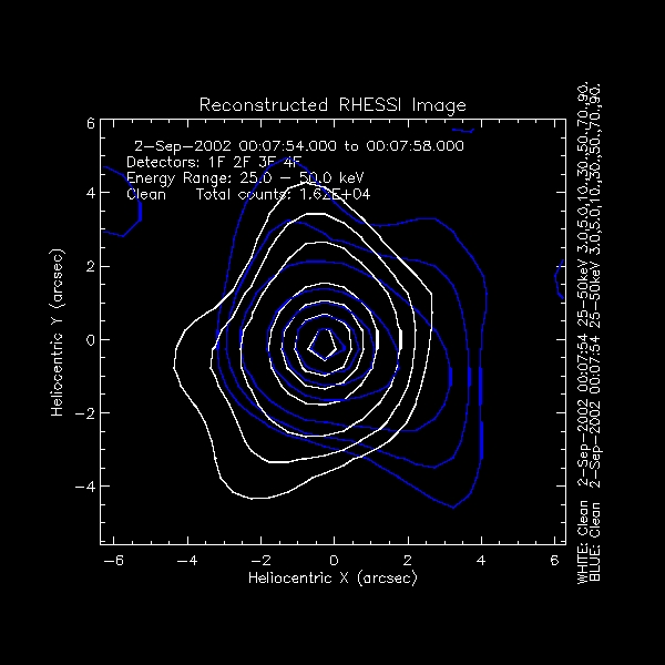
Using detectors 1 - 4, then translating the image of the source near the limb to disk center, we can observe that the 90 % contour to the 30% contour match for both images. The contours for the image at the center extend toward the limb as they go down in level. The image created for the source on the limb does not show foreshortening in along the North - South Heliocentric Y axis. Using the Clean imaging algorithm it is not possible to see the small structure (2 arcsecs and below) differences in the compact source near the limb versus at disk center. The lower level contours do show a distortion toward the disk center for the source near the limb, however I can't determine if this is due to the low number of counts away from the compact source or if it is a demonstration of the displacement of the extended source toward the center of the disk.
The two plots below show the profiles of the the two images. The red curves are the observed data, the white curves are the fits to that data. The first plot shows the profiles of the image at disk center. The second plot shows the profiles of the image near the limb.
The profiles for both images show a bad fit for detectors 1 and 2. The C statistic in each case is over 2.0. This may be a result of the inability of the finer grids to image a source which is extended due to the albedo contribution, but I'm not sure. For detectors 3 and 4 the fits for the image at disk center are good, they each have a C statistic below 1. For the image near the limb the C statistics are above 1. This implies that when the extended albedo source is displaced from the point source detectors 3 and 4 still have trouble imaging both sources while for a source at the center they can create a good image. The caveat to this conclusion is the pointsource and albedo at the center has 1/3 as many total counts as the one on the limb, so this may be a function of bad statistics.
The plot below shows the profiles along a line parallel to the Heliocentric X axis through the source for both images. The source near the limb has been translated so the peak matches the peak at disk center. It has also been normalized so the peak of the profile on the limb matches the flux of the peak at disk center. This was done to make direct comparison of the two profiles easier visually. The red curve is the profile of the image of the source at disk center. The green curve is the profile of the source near the limb.
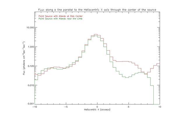
As expected from the contours the profiles match well at the peak off the profile. The distortion in the contours of the image near the limb toward the center are not significant enough to show up in this plot because the levels of those contours are low, however the distortion in the contours of the image at the center toward the limb do appear as an approximately 20% difference toward the limb. This may be a result of only using detectors 1 - 4. This is something I will explore further.
Pixon
The following plot shows the contours of an image for a point source at the center of the disk created using Pixon with detectors 1 -4 compared with a point source near the limb using detectors 1-4 created with Pixon as well. The blue contours are the point source with albedo at disk center, the white contours the point source near the limb.
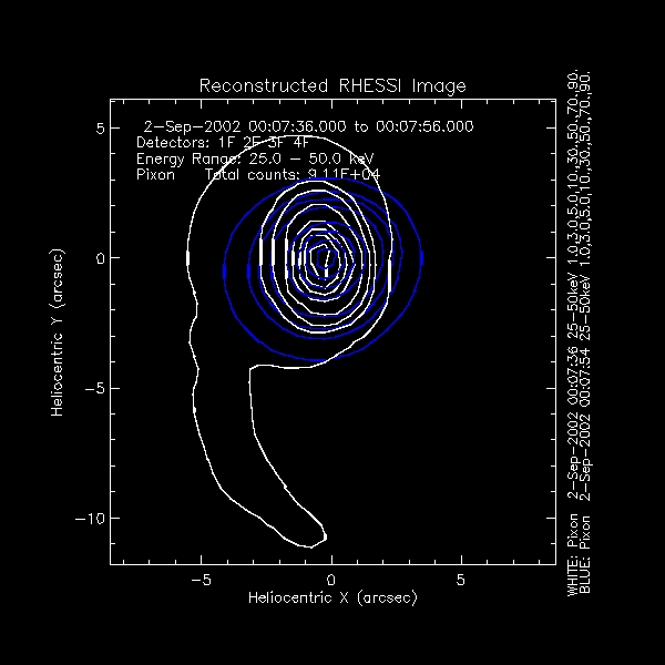
Comparing the point source at the center to that on the limb, the contours of the source at the center are circular while the contours of the source on the limb are extended along the North - South axis and shrunk along the East - West axis. The lowest level contour for the image near the limb is shifted toward the center of the disk.
The plot below shows the flux profiles of the image at the center and the image near the limb along a line parallel to the Heliocentric X axis. The red curve is the profile of the image at the center of the disk. The green curve is the profile of the image near the limb.
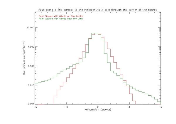
The red curve, showing the profile of the source at the center, is symmetric around the point source and shows the spreading of the gaussian source due to the albedo. This is the expected characteristic spreading of point source at the 10% percent of the peak due to albedo effects. The green curve shows the profile of the source near the limb. Down to 10% of the peak value it is slightly smaller than the full width half max of the original point source. At this point when the original albedo effect seems to appear there is a definite trend showing more flux towards thee heliocentric center. This could be a case of imaging the foreshortening of the albedo, however at the 1% level of the peak value the profile extends toward the limb at a higher level than the profile of the image at the center. These effects need to be looked at with simulations including larger point sources and varying percentages of albedo. The foreshortening effect is predicted and Pixon may be able to image it but the lengthening at the 1% level is a concern if we think real physics can be inferred from those contours. It is possible that the effect is due to the simulation having lower count rates at this level.
The C statistics for both cases were around 1.0 for all detectors, the plots are not included because they were lost in a computer crash. I'll recreate and add them.
UV Smooth
VIS Forward Fit
Forward Fit
Reconstructing Images for Simulated Sources
I've started writing an IDL program to reconstruct an image using a user chosen algorithm and calculate the difference between the reconstructed image and the original data map by doing a pixel by pixel comparison. Right now I'm trying to do this using Eduard Kontar's simulated data because it is the only set for which I have the original data maps. Here is the preliminary version of the program.
Using CASA Algorithms to create Images with RHESSI Data
Brian has decided that this may be a larger and more complicated project than can feasibly be done at present time. I have sent an email to the CASA software group to check on the form our data would need to be in for someone to continue this project.
Assisted visiting student Weishun Liu
I assisted a visiting graduate student from Montana State University with using the OSPEX software to fit RHESSI spectra. I also tried to help her with problems relating to her SSW Installation and upgrade. Those problems were solved with the help of Kim Tolbert and Laszlo Etesi.
