Weekly Report 13Aug2010

From RHESSI Wiki

Revision as of 21:03, 13 August 2010 by Agopie (Talk | contribs)
Jump to: navigation, search

Contents

Weekly Report 13Aug2010

Comparison of a point source with albedo at disk center and a point source with albedo near the limb

The following is a comparison of a simulated point source with albedo at disk center and a simulated point source with albedo near the limb of the sun. In each case the same imaging technique was used to image the source at disk center and on the limb with identical starting parameters. The differences were the eventlist file used in each case, as one had been separately created for each case, and changing the image center so the field of view would include the source.

Clean

The image below shows the contours for two clean images. The blue contours are for the point source with albedo at disk center. The white contours are the point source with albedo near the limb. This image has been translated so that the 90% contour matches the 90% contour at disk center. Both images were made using detectors 1 - 4.
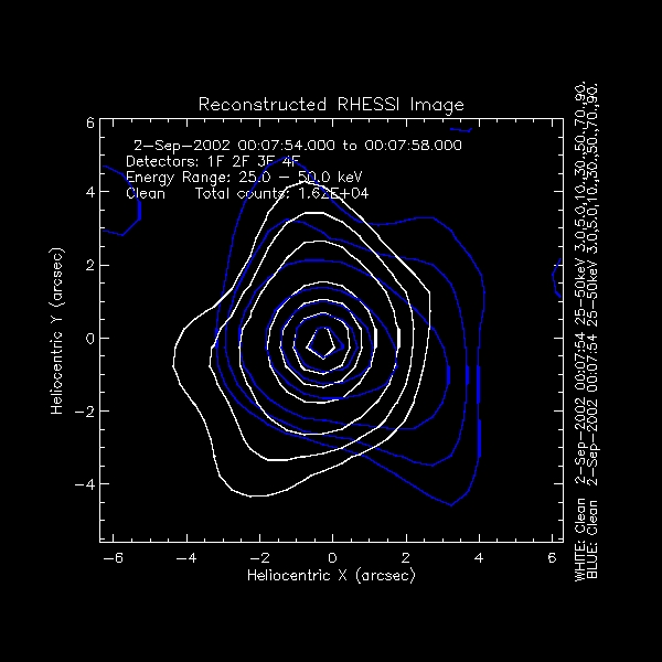
Contours of two clean images. The blue contours are the clean image of a point source with albedo at disk center. The white contours are a clean image of point source with albedo near the limb. It has has been translated to disk center so the 90% contour matches the 90% contour of the image at disk center. Detectors 1 thru 4 were used to create both images.
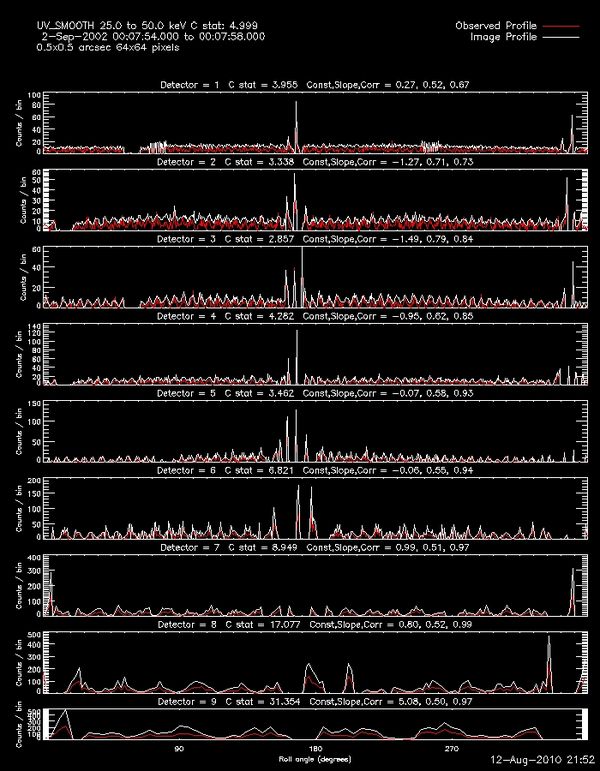
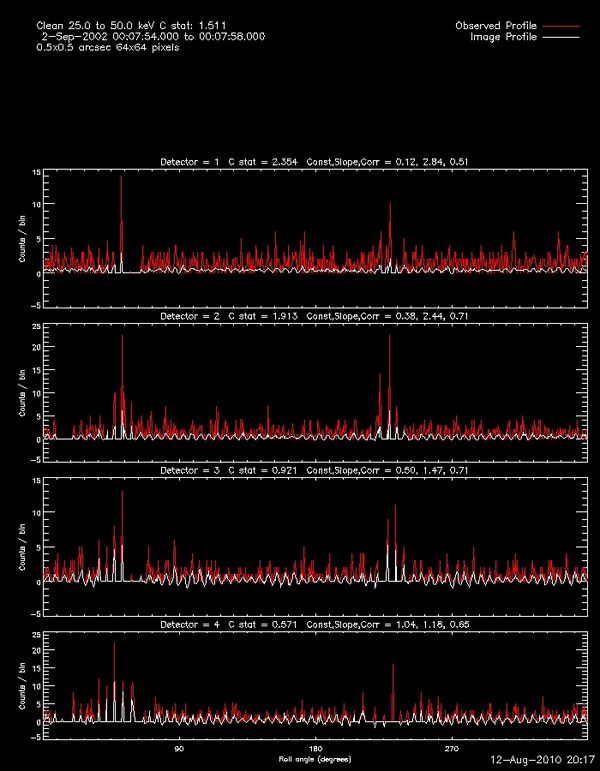
The profiles of the data in each detector used to create the image at disk center along with the fits to those profiles. The data is shown in roll bins.
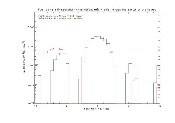
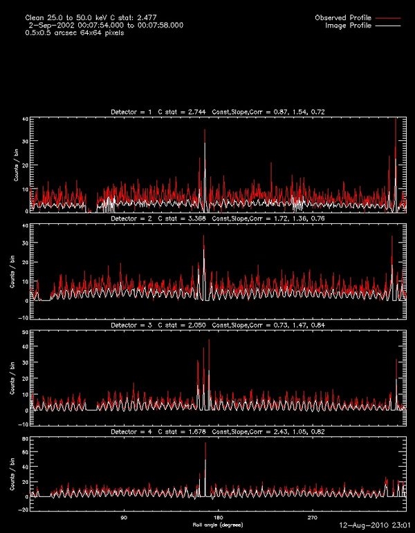
The profiles of each detector used to create the image near the limb along with the fits to those profiles. The data is shown in roll bins.
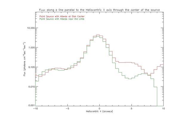
The Flux profiles of each image along a line parallel to the Heliocentric X axis passing through the peak of the source. The red curve is the profile of the image at disk center. The green curve is the profile of the image near the limb. Note the green curved has been divided by a constant so the peak value is near the peak value of the red curve. It has also been translated to disk center. This was done to make it easier to compare the features of the two curves.

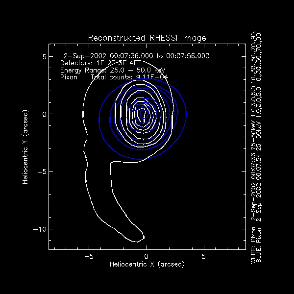
Pixon

Contours of two Pixon images. The blue contours are the Pixon image of a point source with albedo at disk center. The white contours are the Pixon image of a point source with albedo near the limb.It has has been translated to disk center so the 90% contour matches the 90% contour of the image at disk center. Detectors 1 thru 4 were used to create both images.
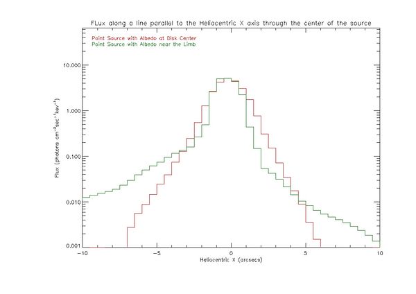
The Flux profiles of each image along a line parallel to the Heliocentric X axis passing through the peak of the source. The red curve is the profile of the image at disk center. The green curve is the profile of the image near the limb. Note the green curved has been divided by a constant so the peak value is near the peak value of the red curve. It has also been translated to disk center. This was done to make it easier to compare the features of the two curves.

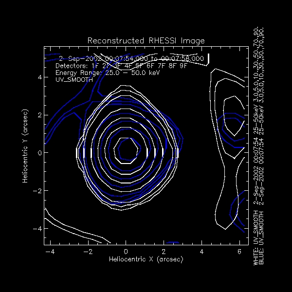
UV Smooth

Uvsmooth blue center white limb.jpg
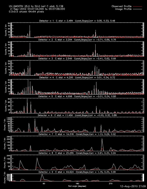
Uvsmooth profiles d1 d9 center.jpg
Uvsmooth profiles d1 d9 limb.jpg
Uvsmooth d1 d9 limb center profile.jpg

VIS Forward Fit

Forward Fit

Reconstructing Images for Simulated Sources

I've started writing an IDL program to reconstruct an image using a user chosen algorithm and calculate the difference between the reconstructed image and the original data map by doing a pixel by pixel comparison. Right now I'm trying to do this using Eduard Kontar's simulated data because it is the only set for which I have the original data maps. I'll put my preliminary version on the Wiki on Monday when I get back to town.

Using CASA Algorithms to create Images with RHESSI Data

Brian has decided that this may be a larger and more complicated project than can feasibly be done at present time. I have sent an email to the CASA software group to check on the form our data would need to be in to use their imaging software. I'm waiting for a response.

Assisted visiting student Weishun Liu

I assisted a visiting graduate student from Montana State University with using the OSPEX software to fit RHESSI spectra. I also tried to help her with problems relating to her SSW Installation and upgrade. Those problems were solved with the help of Kim Tolbert and Laszlo Etesi.
Personal tools
Namespaces
Variants
Actions
Navigation
Toolbox